experience-lab.github.io
Dynamical Systems and Bifurcations
Table of Contents
A dynamical system is a way of talking about a system evolving in time. It is composed of a space of configurations and a prescription for the time evolution of those configurations. One class of dynamical systems describes the configuration as a vector v in some n-dimensional vector space V and specifies the time evolution by giving a formula for the rate of change of v which looks like
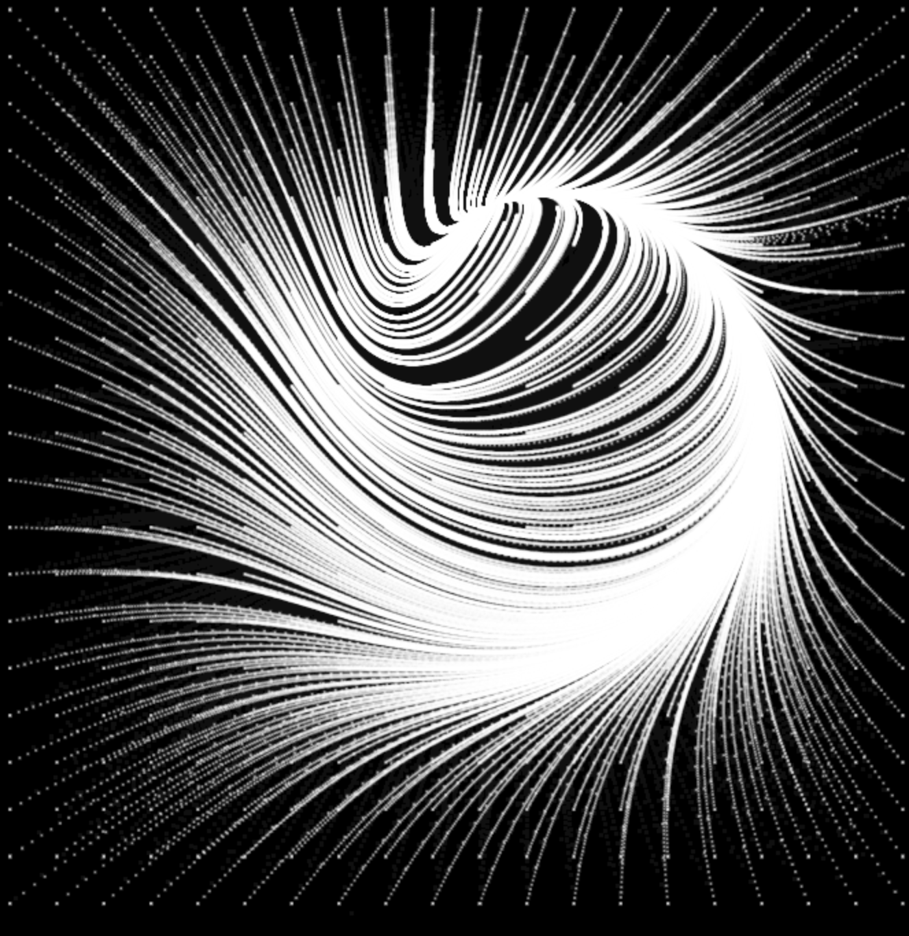
where f is a function from V to V. It can be useful to picture f as a vector field on V, like the velocity field of a fluid. This equation then says that the system moves as would a mote in the flow. We can visualize this when n is small, even drawing the paths of several motes at once, which would represent the fate of several initial configurations simultaneously, and tracing out their streamlines, which represents the history of the configuration.
Hopf Bifurcation
Here is an example which was created using the Hopf bifurcation with the motes intially arranged as an evenly spaced grid. As the time progresses, they are caught up in the flow and pulled towards the circular eddy.
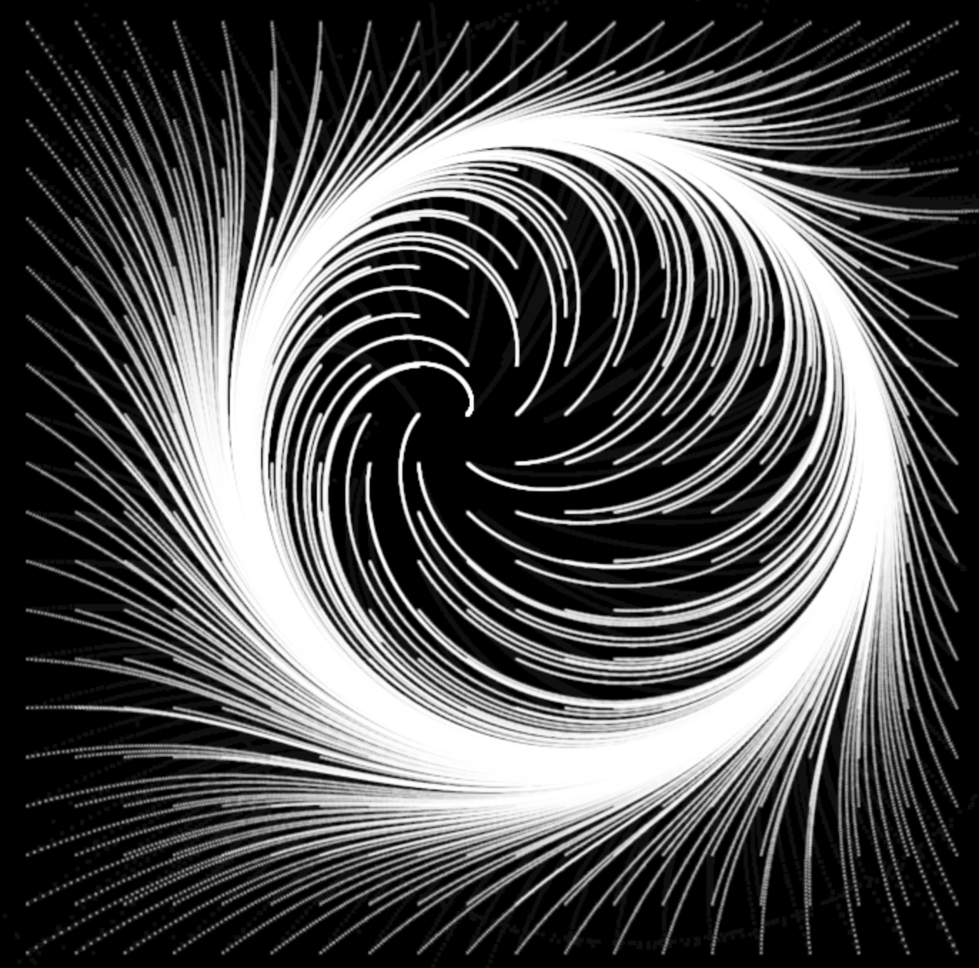
This circular eddy is an example of a limit cycle. In this case it is an attractive limit cycle, meaning nearby points are sucked into its orbit. Systems with attractive limit cycles exhibit spontaneous oscillation. For example, the air blown into a woodwind instrument or across a blade of grass excites a spontaneous oscillation of the reed and can be turned into music by tuning the resonant cavity of the instrument.
This phenomenon can be simplified by considering a fluid flowing in a plane perpendicular to an infinitely long cylinder. Here is a video from the American Physical Society’s Gallery of Fluid Motion which nicely shows the progression from a steady flow to an oscillating flow:
Although the system has infinitely many variables (its configuration is itself a vector field) and displays intricate phenomena including turbulence, the transition from steady to oscillating can be understood in a two-variable model called the Hopf bifurcation. Transitions like these in dynamical systems are generally called bifurcations and the classification of bifurcations is a problem in topology.
Here is the simulation of the Hopf bifurcation.
It is modelled with three parameters a, b, and c (real numbers).
- a is the tuning parameter of the bifurcation: when a <= 0, the system has a stable fixed point - every starting configuration eventually spirals into this stationary state. When a > 0, this fixed point becomes unstable and “emits” a stable limit cycle - almost every starting configuration will eventually join this oscillating cycle.
- b controls the sign and strength of circulation. It is 1 by default.
- c adds a constant velocity along the x axis. When c begins to overpower the circulation b, there are new bifurcations and the limit cycle can be destroyed.
We can compactly express the time evolution equation by expressing the configuration (a point in the 2d plane) as a complex number z: